With progress well underway for the actual satellite itself—both in hardware and firmware— we’ll now move on to our wildfire modeling simulation.
Modeling FIREEEEEE
Data Processing
Only two data points are received from the satellite that are of use to the simulation, geolocation data, and the actual picture from the satellite. This data must be processed into a format usable by the computer.
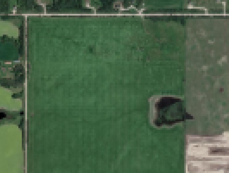
From the image we are able to extract moisture, and packing ratio (the material and its density). Since the image has many more pixels than what we’d like to simulate, the image is chunked into 133x100 blocks. Using some simple trigonometry the actual size of each of these blocks can be calculated. The FOV of the camera is known at 62.2° by 48.8°, so from 1km in the air the total dimensions of the image are 1.2km by 0.907km. Dividing by the previously established image chunking dimensions for each axis, we get a unit size of about 9.07m! This is irrelevant to the actual simulation calculations, but gives a good idea on the expected precision of the end result.
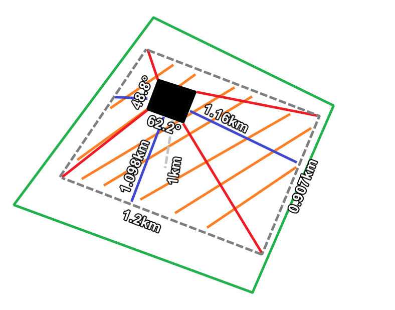
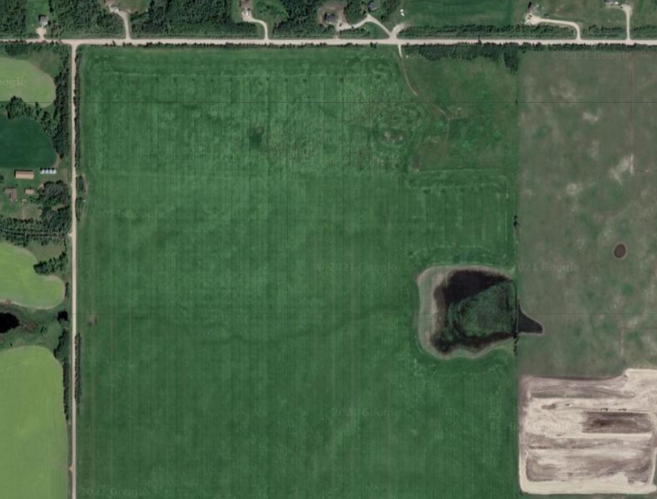
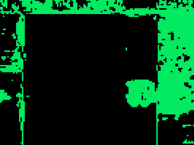
Within each of these blocks the average color is taken to obtain the required values. For example the moisture content is found by analyzing how “dry” of a color the square is. We establish what “dry” means by examining mostly the green value, however the other colors are also important. If we were to ignore the other colors we would assume all squares with 255 green are super moist, but what if the red value was also 255? Then we wouldn’t have a super moist section of ground, we might have someone’s pumpkin field! This is done in Python specifically the Pillow image processing library
| Sample Image | Data Chunks | 30% Moisture Content Analysis |
|---|---|---|
 |
 |
 |
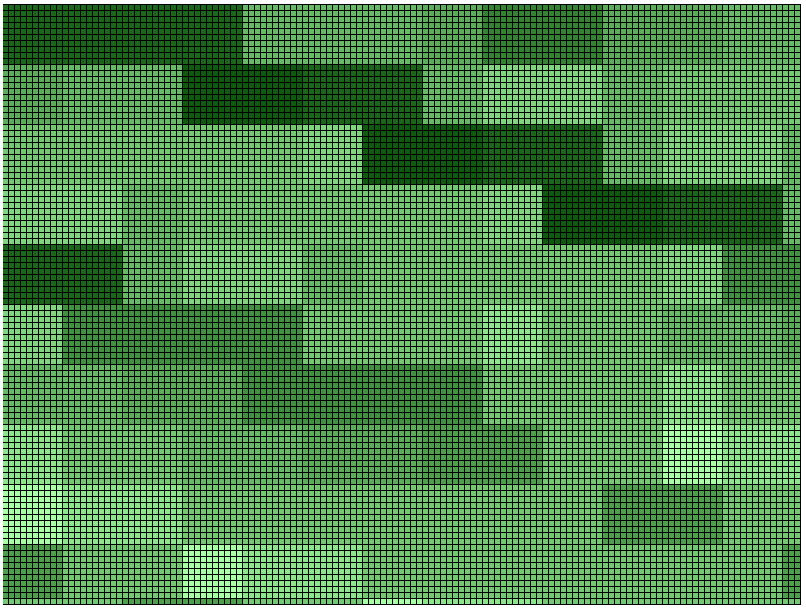
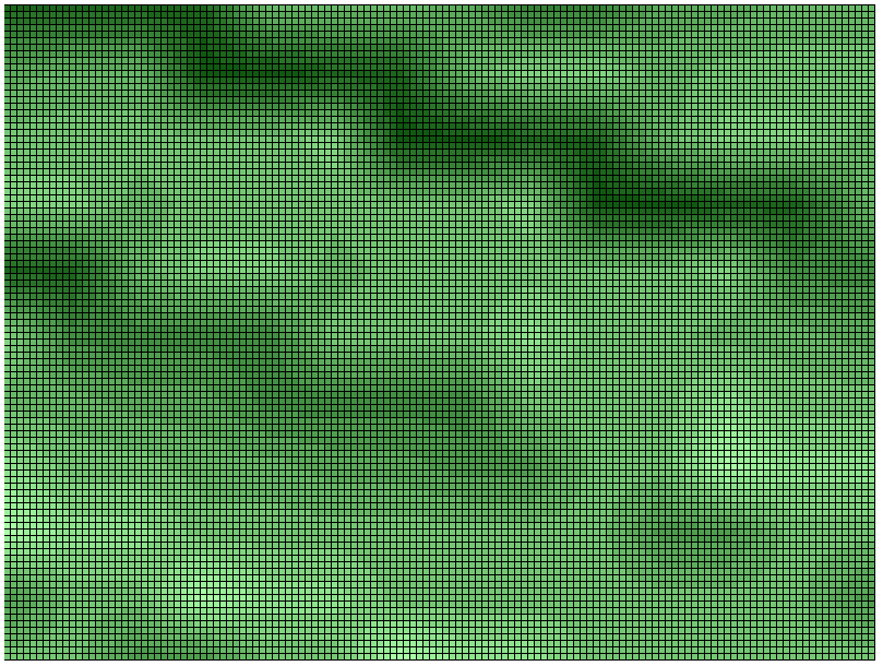
Elevation data is not recorded by our satellite and as such must be sourced from an external source. Thankfully the location of our satellite is recorded with a GPS module so we are not totally in the dark. By using the Open-Elevation (https://open-elevation.com/) API, we are able to find the elevation at any point on the globe. So to find the elevation across our image we must find a set of points that span across our image. This is a more complicated task than it seems. Latitude and longitude are measurements derived as the angle from the equator and prime meridian respectively, as such there is not a one to one correspondence that we can add to get a grid of geolocation points across our image. Thankfully there exists a library that makes latitude and longitude calculations easy https://github.com/chrisveness/geodesy. The elevation API does not have infinite precision, so we only find a coordinate point every 90 meters. After finding the grid of coordinates the API returns the elevation at each point. This gives us the elevation above sea level in a 90 meter block grid across the image. We can improve this blockiness with interpolation. Specifically we use bilinear interpolation to smooth the edges and provide more of a gradient between the elevation points. This can be seen in the below two images, the first being the data we get from the API, and the second being after interpolation, this method allows us to estimate the real elevation of points outside of the level of precision that the API has.
 |
 |
The values measured for each property are then put into a json file for the simulation to use.
Simulation
Now how do we simulate a fire? Well an article published in the International Journal of Modeling and Optimization provides a simple calculation.
\(\begin{aligned}
\text{FSR} &=
\begin{bmatrix}
(0.0002\text{ FMC}^2-0.008\text{ FMC}+0.1225)V^2\\
+(-0.0008\text{ FMC}^2+0.0005\text{ FMC}+0.1823)V\\
+(0.0019\text{ FMC}^2-0.0924\text{ FMC}+1.2675)\\
\times \beta_a \times (\beta_s+1)
\end{bmatrix}\\\\
\beta_a&=0 \text{, if } \alpha =0\\
\beta_a&=(0.0075\alpha^{-0.196})V^2+(0.0002\alpha-0.0985)V+4.0767\alpha^{0.429}\\
\\
\beta_s&=5.275\beta^{-0.3}(\tan(\varphi ))^2\\\\
\text{FSR}&=\text{Fire Spread Rate (ft/min) in a particular direction}\\
\text{FMC}&=\text{Fuel Moisture Content}\\
V&=\text{Wind Speed (mi/h)}\\
\\
\beta_a&=\text{Angle Ratio}\\
\alpha&=\text{Angle between the direction of the FSR being}\\
&\text{calculated and the direction of the wind (degrees)}\\
\\
\beta_s&=\text{Slope Factor}\\
\beta&=\text{Packing Ratio}\\
\varphi&=\text{Slope of the fuel bed, so that }\tan(\varphi)\text{ = rise/run}
\end{aligned}\)
Oops, maybe not so simple looking, but I assure you the input is quite simple. By inputting moisture, packing ratio, the direction of the wind and the incline of the slope (how much the elevation changes from one end to another). The equation returns the rate of spread in feet per minute of the fire. For the sake of simplicity a unit can set other units of fire when it is fully on fire. As such the simulator steps can be done as follows:
- Check for units within a 1 unit distance for other units on fire
- Calculate the fire spread rate
- Update how much the unit is on fire
- Update how much left the unit can burn
- Repeat steps 1-4
 |
 |
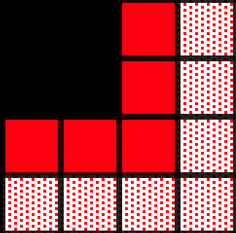 |
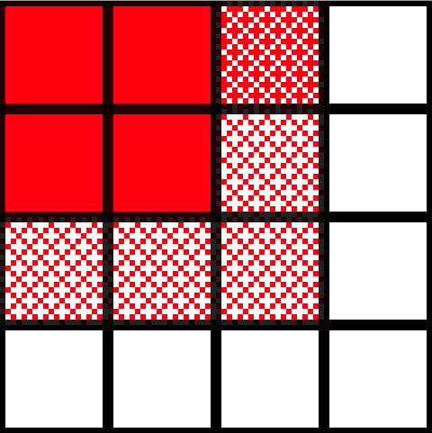
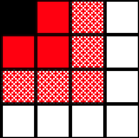
An example of how the cycles play out can be found in the above images. In the first image the units in the top left spread their fire to the other units. In the second image one of the units burns out, while the fire spreads within the other units. In the last image, the fire has fully spread within the previous units and can now spread to the next units.
We wanted the simulator to be easily accessible, and to achieve this we the simulation is written in Javascript enabling it to be run client side on a web browser, meaning anyone can access it without downloading anyfiles.
Renderer
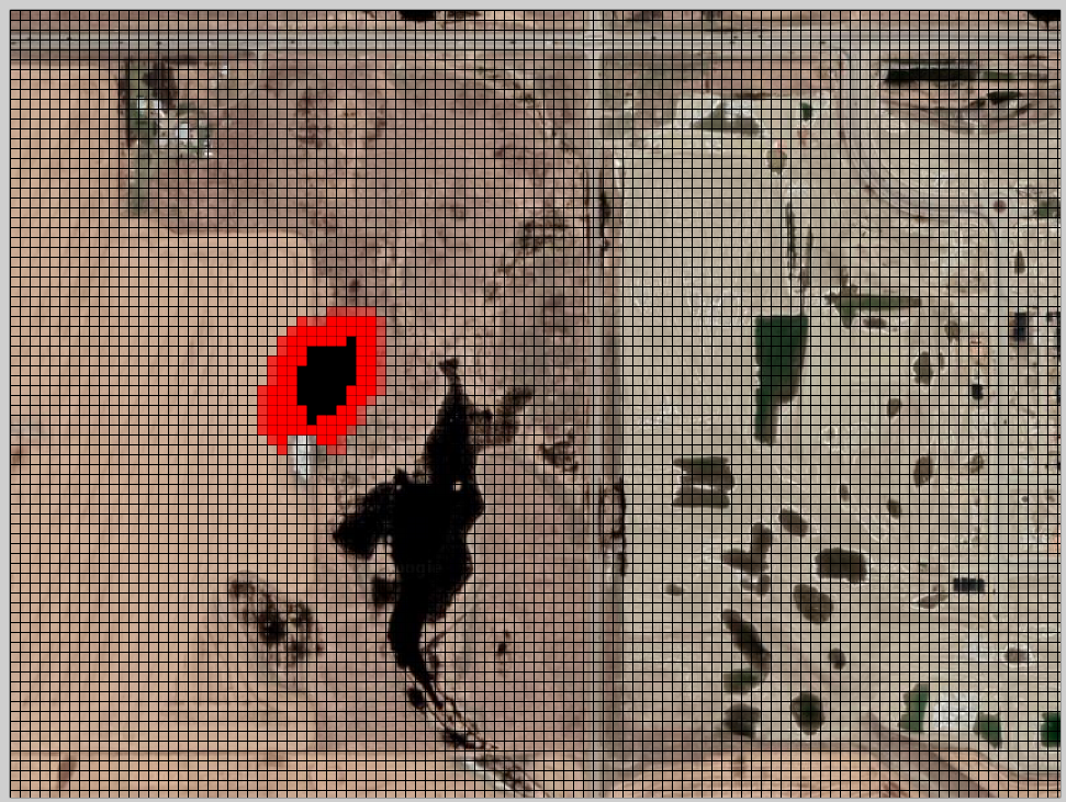
The simulator only simulates values and returns more numbers! The user has no way of visualizing the data directly from the simulator. That is where the render comes in, using PixiJS (https://pixijs.com/) a WebGL based HTML5 graphic library the data can be displayed to the user. The render reads the array of the current state of all the simulation units and shows the user what units are on fire, not on fire, previously on fire, and currently burning.
UI
The user interface is very simple, allowing the user to start/stop the simulation. And adjust two specific variables, the wind direction, and where the fire starts. This is designed using Vue.js which is a component based Javascript framework, which eases UI design and allows for quick creation of interactive and responsive website designs.
That’s all we have for now! Stay tuned to see the simulator pop up on the website, and maybe even more blog posts explaining certain aspects in further detail!